Lagrange interpolation
| table of contents | |
|---|---|
| - | Lagrange interpolation |
| - | Example 1: Linear interporation |
| - | Example 2: Quadratic interpolation |
| - | Example 3: Cubic interpolation |
| - | Uniqueness |
Lagrange interpolation
Let $f(x)$ be an arbitrary real function.
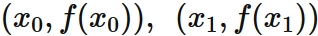
The nth degree polynomial passing through $n + 1$ points

Proof
Let
$$
\tag{1}
$$
be $n+1$ points on a real function $f(x)$, where
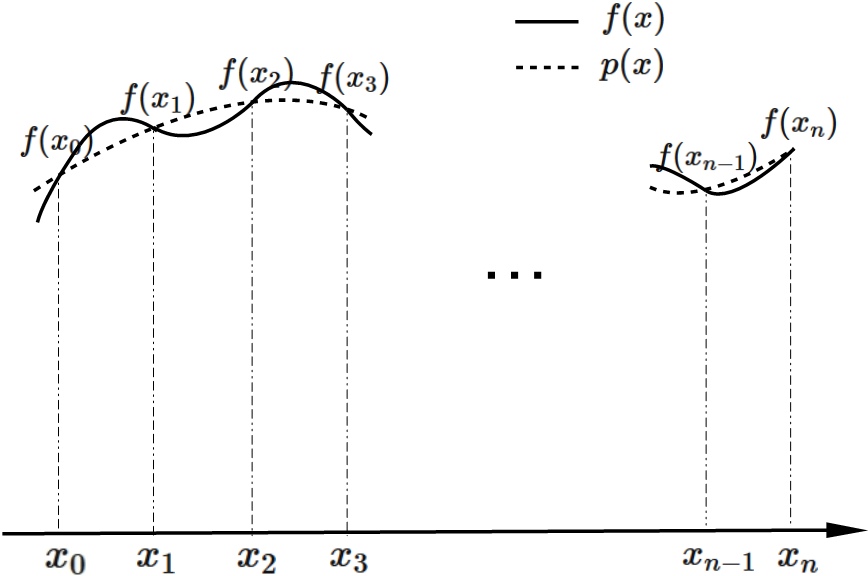
 Let $p(x)$ be the nth degree polynomial passing through $(1)$. $p(x)$ satisfies
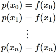 $$
\tag{2}
$$
(See fig. below).
$$
\tag{2}
$$
(See fig. below).
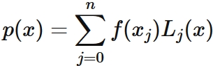
 We put $p(x)$ as
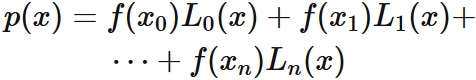 $$
\tag{3}
$$
, where $L_{i}(x)$ $(i=0,1, \cdots,n)$ are nth degree polynomials.
(The specific form of $L_{i}(x)$ has not been determined at this point.)
$$
\tag{3}
$$
, where $L_{i}(x)$ $(i=0,1, \cdots,n)$ are nth degree polynomials.
(The specific form of $L_{i}(x)$ has not been determined at this point.)
If $L_{i}(x)$ satisfy
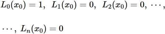 ,
$p(x_{0}) = f(x_{0}) $.
If $L_{i}(x)$ satisfy
,
$p(x_{0}) = f(x_{0}) $.
If $L_{i}(x)$ satisfy
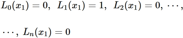 $p(x_{1}) = f(x_{1}) $.
In the same way, we see that
if $L_{i}(x)$ satisfy,
$p(x_{1}) = f(x_{1}) $.
In the same way, we see that
if $L_{i}(x)$ satisfy,
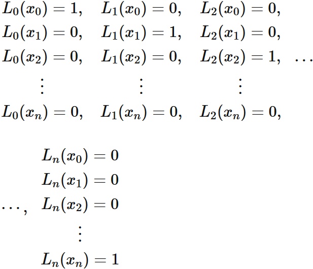 $$
\tag{4}
$$
, $p(x_{j}) = f(x_{j})$ $(j=0,1,\cdots,n)$.
$$
\tag{4}
$$
, $p(x_{j}) = f(x_{j})$ $(j=0,1,\cdots,n)$.
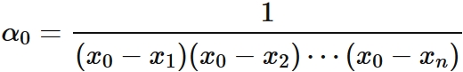
In $(4)$, $L_{0}(x_{i}) = 0$ for $i =1, 2, \cdots, n$. By the factor theorem, $L_{0} (x)$ can be expressed as
 , where $\alpha_{0} $ is a constant.
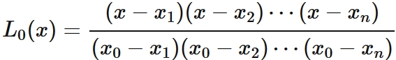
By $L_{0}(x_{0}) = 1$, it is derived as
, where $\alpha_{0} $ is a constant.
By $L_{0}(x_{0}) = 1$, it is derived as
 Therefore we obtain
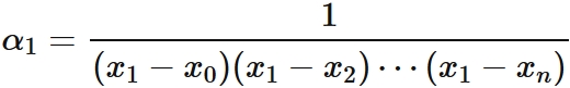
In a similar way, since $L_{1}(x_{i}) = 0$ for $i =0,2,3\cdots,n$, by the factor theorem, we obtain $L_{1}(x)$ can be written as
 , where $\alpha_{1} $ is a constant.
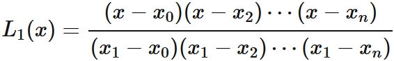
By $L_{1}(x_{1}) = 1$, it is derived as
, where $\alpha_{1} $ is a constant.
By $L_{1}(x_{1}) = 1$, it is derived as
 .
Therefore we obtain
.
Therefore we obtain
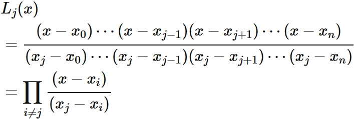
 By repeating the same discussion,
we can derive $L_{j}(x)$ for $j = 0,1,\cdots, n$ as
By repeating the same discussion,
we can derive $L_{j}(x)$ for $j = 0,1,\cdots, n$ as
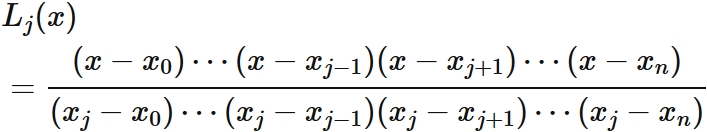 .
This expression can be written by the symbol $\prod$ as
.
This expression can be written by the symbol $\prod$ as
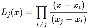 $$
\tag{5}
$$
$$
\tag{5}
$$
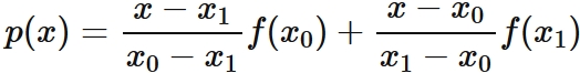
Substituing $(5)$ into $(3)$, we have
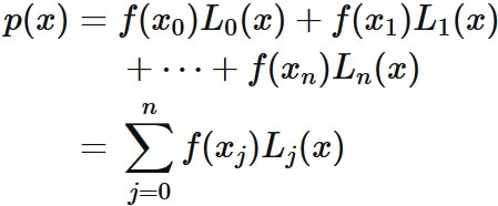 It is clear that this function passes through points $(1)$ (that is, it satisfies $(2)$), since $L_{j}(x)$ satisfies $(4)$.
Approximating the original function $f (x)$ with the polynomial function $p (x)$ defined in this way, that is,
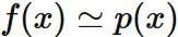 is called Lagrange interpolation.
Let
If $L_{i}(x)$ satisfy
In $(4)$, $L_{0}(x_{i}) = 0$ for $i =1, 2, \cdots, n$. By the factor theorem, $L_{0} (x)$ can be expressed as
In a similar way, since $L_{1}(x_{i}) = 0$ for $i =0,2,3\cdots,n$, by the factor theorem, we obtain $L_{1}(x)$ can be written as
Substituing $(5)$ into $(3)$, we have
Approximating the original function $f (x)$ with the polynomial function $p (x)$ defined in this way, that is,
Lagrange's interpolation is
a formula for finding a polynomial that approximates the function $f(x)$,
but it simply derives a nth degree function passing through $n + 1$ given points.
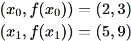
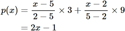
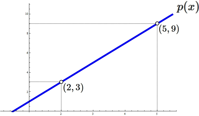
Example 1: Linear interpolation
Let $f (x)$ be a function that passes through two points
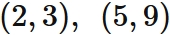
Answer
Lagrange's interpolation formula that gives the linear function passing through two points
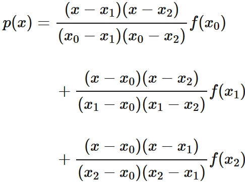
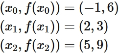
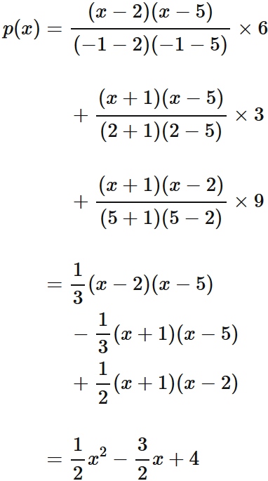
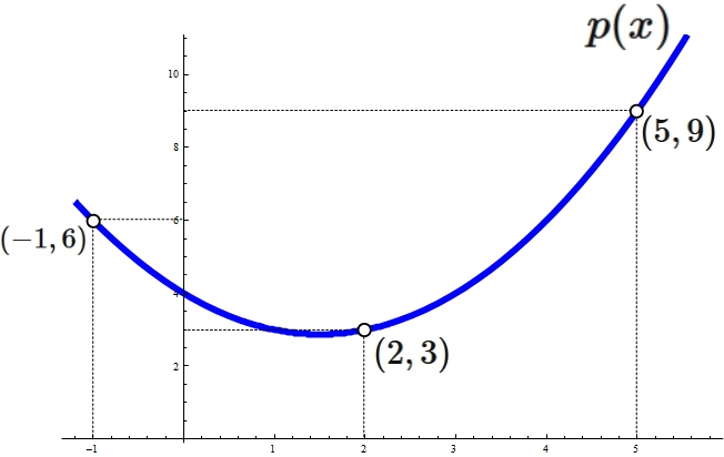
Example 2: Quadratic interpolation
Let $f (x)$ be a function that passes through three points
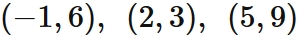
Answer
Lagrange's interpolation formula that gives the quadratic function passing through three points

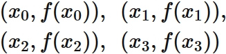
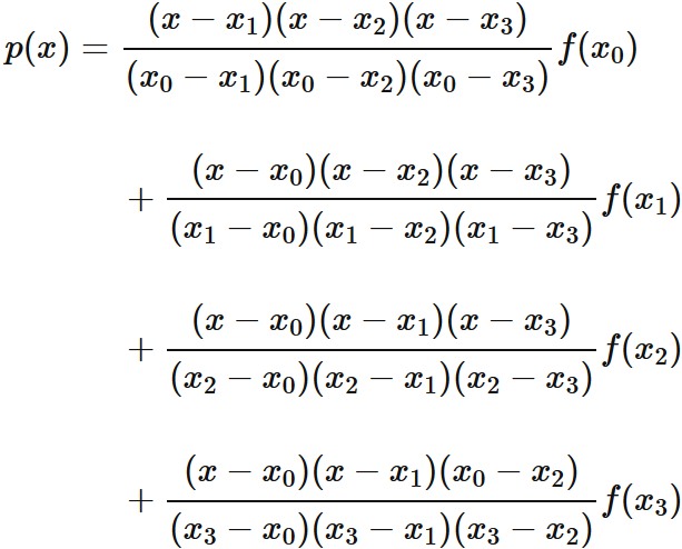
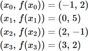
Example 3: Cubic interpolation
Let $f (x)$ be a function that passes through four points

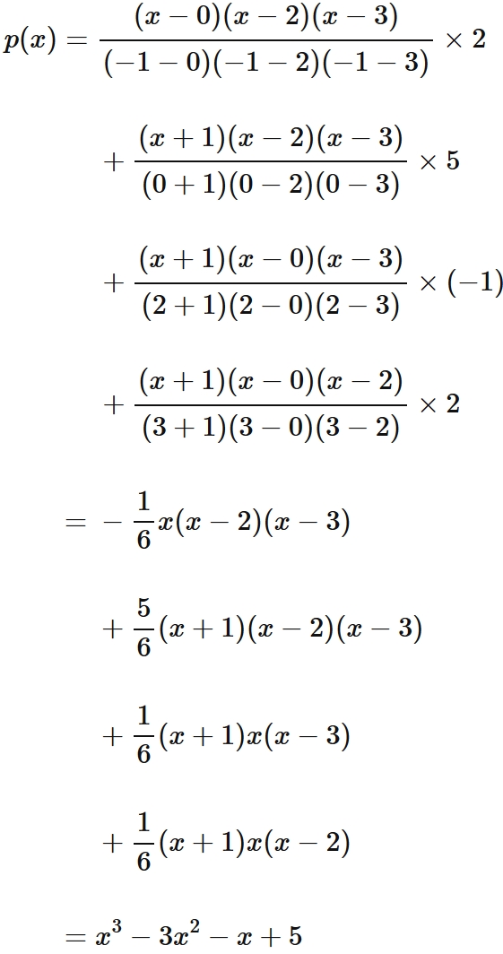
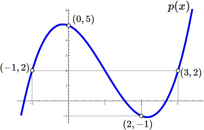
Answer
Lagrange's interpolation formula that gives the qubic function passing through four points
Uniqueness
A polynomial of degree $n$


Proof
Problems solving a system of linear equations
Let $f(x)$ be a polynomial of degree $n$ defined as
, and that passes through $n+1$ different points,
.
We have
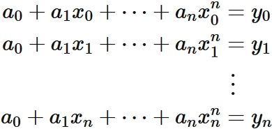 $$
\tag{2}
$$
$$
\tag{2}
$$
Let $X$ be an $(n+1) \times (n+1)$ matrix, and $\mathbf{a}$ and $\mathbf{y}$ be $n$ dimensional vectors defined as
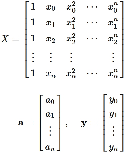 .
Equations $(2)$ can be written as
.
Equations $(2)$ can be written as
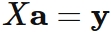 $$
\tag{3}
$$
$$
\tag{3}
$$
Equation $(3)$ ( or $(2)$) is a system of $n+1$ linear equations with $n+1$ unknowns.
A necessary and sufficient condition for the system of linear equations whose coefficient matrix is a square matrix to have a single solution is that the coefficient matrix is a non-singular matrix (a matrix having and inverse matrix). Therefore, if it is shown that the coefficient matrix of $(3)$ is a non-singular matrix, it means that the solution of $(3)$ is unique.
Let us focus on the coefficient matrix $X$. The transpose matrix of $X$ is a Vandermonde matrix
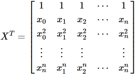 It is known that the determinant of the Vandermonde matrix is given as
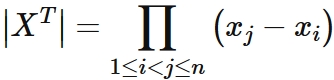 , where $\prod_{1 \leq i < j \leq n}$ means that
all $( x_{j}- x_{i} )$ are multiplied if $1 \leq i < j \leq n$.
Specifically,
, where $\prod_{1 \leq i < j \leq n}$ means that
all $( x_{j}- x_{i} )$ are multiplied if $1 \leq i < j \leq n$.
Specifically,
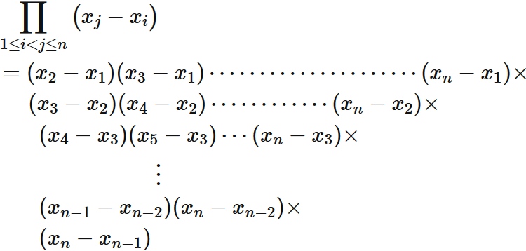
In our discussion, every $x_{i}$ is different. If $i \neq j$, $x_{i} \neq x_{j}$. We have
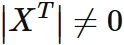 Generally, the determinant of the transposed matrix is equal to the determinant of the original matrix.
We have
Generally, the determinant of the transposed matrix is equal to the determinant of the original matrix.
We have
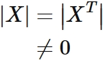 Since a matrix whose determinant is not $0$ is a non-singular matrix, $X$ is shown to be a non-singular matrix.
Problems solving a system of linear equations
Let $f(x)$ be a polynomial of degree $n$ defined as
Let $X$ be an $(n+1) \times (n+1)$ matrix, and $\mathbf{a}$ and $\mathbf{y}$ be $n$ dimensional vectors defined as
Equation $(3)$ ( or $(2)$) is a system of $n+1$ linear equations with $n+1$ unknowns.
$X$ is non-singular
In order for the function $f (x)$ to be unique,
each coefficient $a_{0}, a_{1}, \cdots, a_{n}$ must be unique.
To be so,
the solution of system of linear equations $(2)$, that is $\mathbf{a}$, must be unique.
A necessary and sufficient condition for the system of linear equations whose coefficient matrix is a square matrix to have a single solution is that the coefficient matrix is a non-singular matrix (a matrix having and inverse matrix). Therefore, if it is shown that the coefficient matrix of $(3)$ is a non-singular matrix, it means that the solution of $(3)$ is unique.
Let us focus on the coefficient matrix $X$. The transpose matrix of $X$ is a Vandermonde matrix
In our discussion, every $x_{i}$ is different. If $i \neq j$, $x_{i} \neq x_{j}$. We have
Conclusion
As described above,
the coefficient matrix $ X $ of the system of linear equations $(3)$
is a non-singular matrix and therefore has the unique solution.
Solving $(2)$ gives the unique coeffient $a_{0}, a_{1} \cdots, a_{n}$.
The function of $f(x)$ is uniquely determined.
Therefore,
a function that passes through different $n+1$ points is unique.